
4.1. Blending
Blending enables continuous motion execution by allowing smooth transitions between consecutive motion commands without stopping at intermediate target positions. The blending behavior is defined retroactively, meaning that the blending parameters of a motion command determine how the transition from the preceding command is executed.
Each motion command can participate in blending with both the preceding and the subsequent command. As a result, the maximum allowable blending radius is constrained to half of the shorter of the two adjacent motion segments.
Basic Requirements
To perform blending, the following basic requirements must be met:
There must be two segments between which blending can be performed.
Both segments must contain movement. Blending is not possible if either segment has no movement.
A blending parameter greater than
0.0must be set.
4.1.1. Blending Overview
The following table summarizes the key differences between PTP blending (see PTP Blending), Cartesian blending (see Cartesian Blending), and PTP-LIN blending (see PTP-LIN Blending):
4.1.2. Cartesian Blending
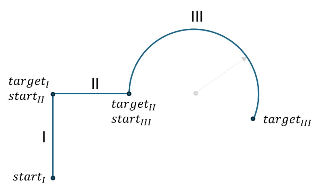
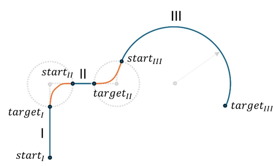
For Cartesian motions, blending is applied to both translation and orientation. During translational blending, a fifth-order polynomial is inserted as an intermediate segment between consecutive motion segments to ensure a continuous path (see Fig. 14). As a result, the robot motion remains continuous and does not stop at the segment transition points.
Fig. 13 illustrates the original Cartesian path with discrete motion segments, while Fig. 14 shows the same path with blending applied. The blending regions between consecutive segments are highlighted to indicate where the transition is smoothed.
Blending Segment
As mentioned earlier, during translational blending, a fifth-order polynomial is inserted as an intermediate segment. The term ‘fifth-order’ refers to the geometry of the path and not to the motion profiles for velocity or acceleration.
If there is no translational path length, pure rotations are blended, meaning there is no translational movement within the blending segment.
The blending segment adopts the velocity and acceleration settings from the adjacent segments. In each case, the lower value of the adjacent segments is used.
In addition, the fifth-order polynomial segment may further reduce the maximum velocity based on it’s curvature.
Cartesian Blending Parameters
The Cartesian blending parameter defines how translation and rotation are blended between consecutive motion segments. It can be specified either in absolute terms \([\mathrm{m}]\) (only for translational blending) or as a percentage \([\mathrm{\%}]\).
Absolute Blending
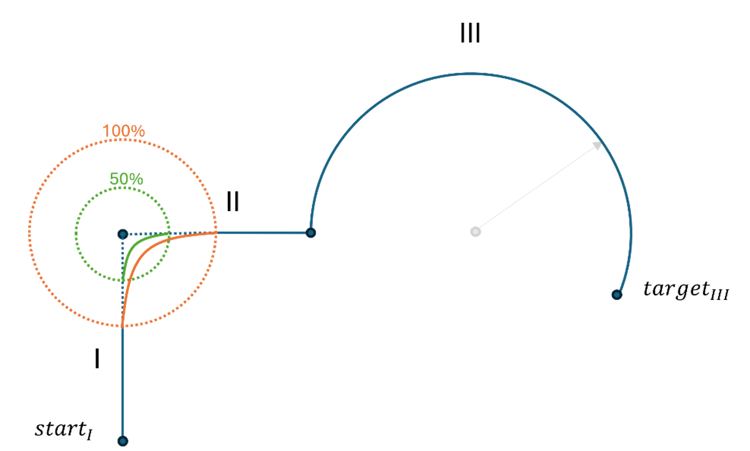
For absolute blending, the parametrized value \([\mathrm{m}]\) is limited to half of the path length of the shorter segment and can only be applied if the segment has a translatory path component. The rotational blending is automatically scaled to match the translational blending radius.
Percentage Blending
Percentage blending always refers to the half of the shorter segment’s path length. In this process, translation and rotation are considered separately.
Blending radius calculation
The blending parameter is internally converted to a blendingfactor in the range \([0.0 \ldots 1.0]\). Based on this, the blending radius is calculated as follows:
Note
Blending parameters that exceed 100% or are longer than the blendable path length are limited to the maximal blendable path length.
Fig. 15 illustrates the blending radii applied to consecutive motion segments. Segment II is the segment with the shorter path length. Therefore, the maximum blending radius is half the path length of Segment II.
Examples for Cartesian Blending
Fig. 16 illustrates the Cartesian path from Fig. 13 with different blending parameter settings. Five cases are shown: no blending (0 %), 25 %, 50 %, 75 % and 100 % blending. As the blending parameter increases, the transitions between consecutive segments become progressively smoother, resulting in a more continuous motion path.
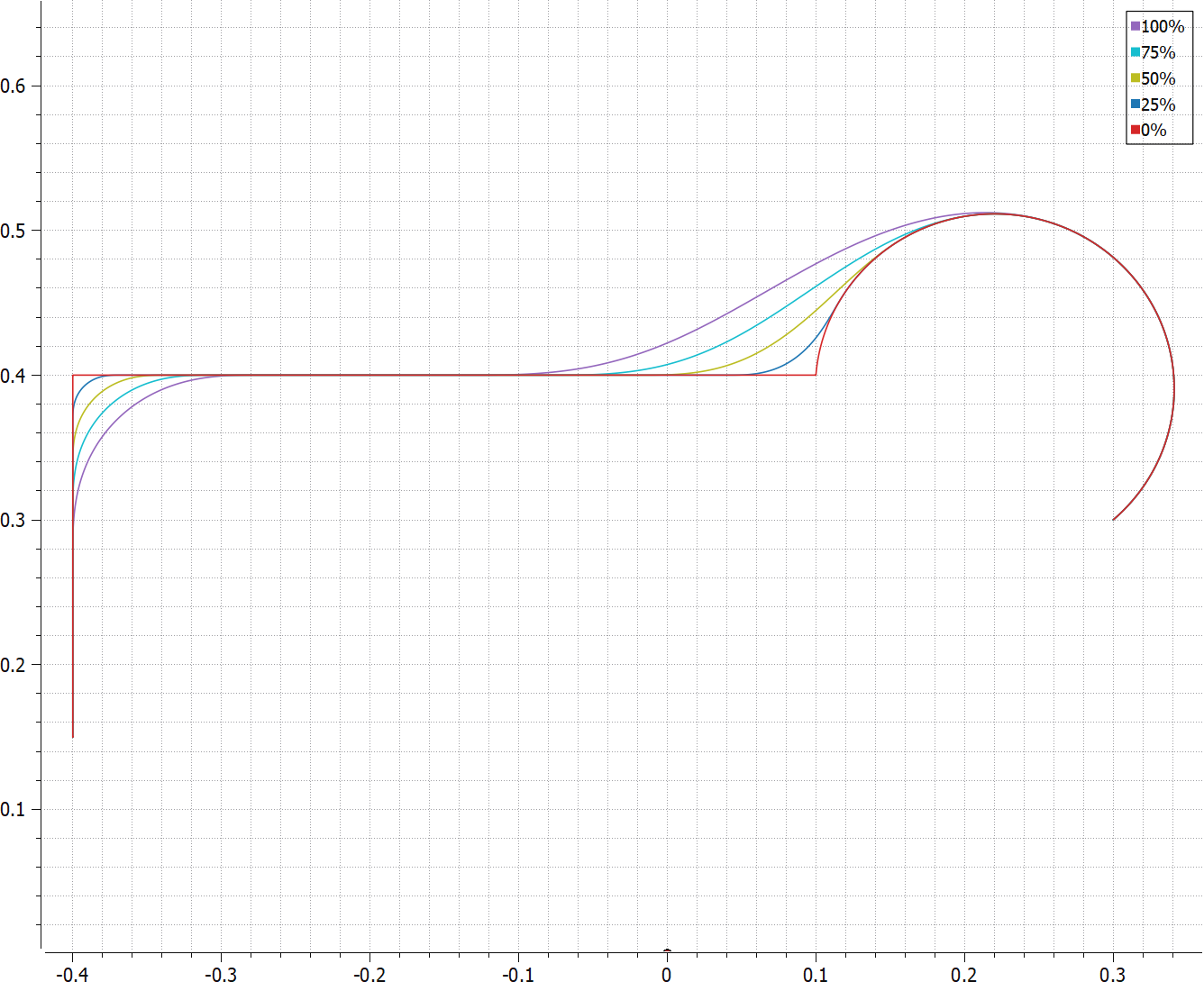
Fig. 16 Example for Cartesian blending with different blending parameters
Edge Cases for Cartesian Blending
This section highlights specific situations in Cartesian blending that require special consideration. These cases demonstrate how the blending behavior adapts under unusual or limiting conditions, ensuring predictable motion even in non-standard scenarios.
Blending in the Opposite Direction
When consecutive motion segments are oriented in opposite directions, the path is shortened according to the blending radius. In this case, no transition velocity is applied between the segments.
Blending in the Same Direction
When consecutive motion segments are heading in the same direction, blending can be used to achieve a transition velocity without coming to a standstill between the segments. Even in this case, a valid blending parameter must still be set.
Blending Parameter
For Cartesian blending, a blending parameter of more than 2.0% must currently be set. Otherwise no blending is
performed, even if the consecutive segments are aligned in the same direction. The motion follows the original discrete
path without smoothing at the segment transitions.
Blending Between Pure Translation and Pure Rotation
It is possible to blend between segments in which, for example, one moves purely translational and the other moves purely rotational.
4.1.3. PTP Blending
For point-to-point (PTP) motions, blending is calculated individually for each axis. The blending coordinate for each axis corresponds to the joint angle:
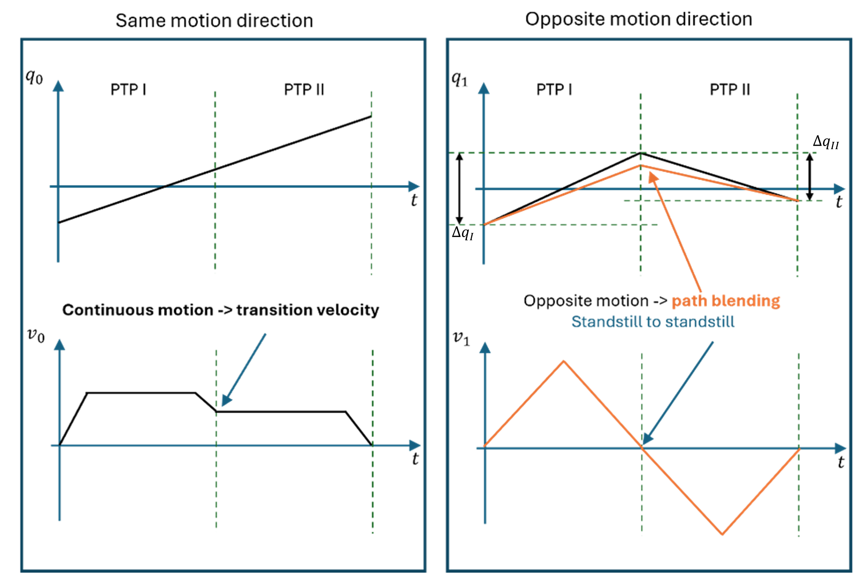
The blending behavior of each axis depends on the motion direction between consecutive segments and can be categorized into three cases: same direction, opposite direction, or no motion in at least one segment.
When the axis continues in the same direction across consecutive segments, it can maintain a transition velocity greater than zero.
In contrast, if the axis reverses direction between consecutive segments, it must stop and change motion direction (transition velocity = 0), but the path can be blended and shortened.
If the axis does not move in at least one segment, no blending is performed for that axis.
Fig. 17 illustrates blending in joint space, highlighting the differences between same and opposite motion directions.
PTP Blending in Same Direction
In contrast to Cartesian blending, a blending parameter of 0.0% is currently sufficient in PTP to achieve a
transition velocity for axis in the same direction.
PTP Blending in Opposite Direction
When blending consecutive PTP commands in opposite directions, the maximum blending radius for each axis corresponds to half of the path length of the shorter segment, similar to the concept of the blending radius described for Cartesian blending, see Cartesian Blending Parameters. Mathematically, the joint space blending distance is calculated as
Fig. 18 illustrates the path lengths of two consecutive PTP commands, \(\Delta q_I\) and \(\Delta q_{II}\).
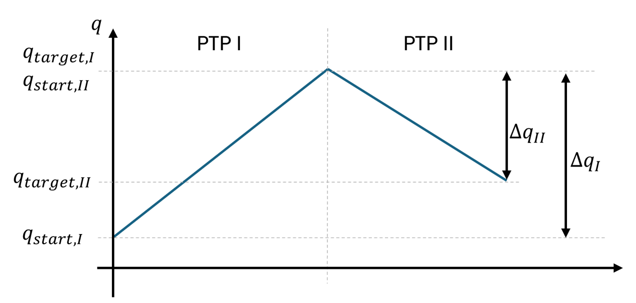
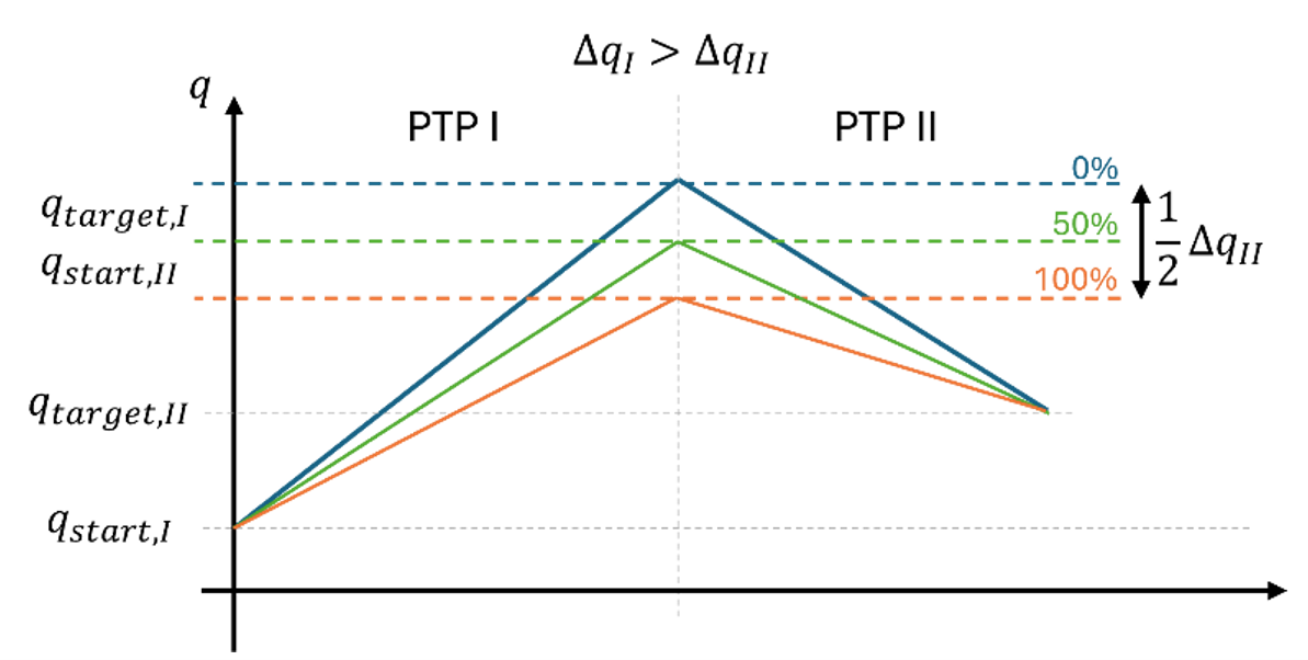
Unlike Cartesian blending, no intermediate segment is inserted in joint space. Instead, the start and target coordinates are adjusted directly according to the calculated blending radius. The adjusted coordinates are computed as
Fig. 19 illustrates the blending radius in joint space, showing the positions of \(q_{\mathrm{start},I}\), \(q_{\mathrm{target},I}\), \(q_{\mathrm{start},II}\), and \(q_{\mathrm{target},II}\) along the motion path.
Examples for PTP Blending
The following example demonstrates the different cases of PTP blending. Two consecutive commands are considered. For axis 1 (A1), the motion continues in the same direction, allowing a transition velocity to be applied; in this case, the path is not shortened. For axis 2 (A2), the motion reverses direction between the two commands. The axis must stop at the segment boundary, but the path is shortened according to the blending radius.
The joint positions for the two commands are as follows:
This results in the following blending cases:
Axis 1 moves in the same direction, so no path shortening occurs.
Axis 2 moves in opposite directions, with PTP I contributing \(30 \mathrm{°}\) and PTP II \(-20 \mathrm{°}\) to the blended path. The resulting blending distance is calculated as
\[\Delta q_{Blend} = \frac{1}{2} \cdot \min \big( |+30|, |-20| \big) \cdot \text{blendingfactor}\]Depending on the selected blending factor, the path shortening is adjusted accordingly: 100 % blending corresponds to a 10° shortening, while 50 % blending results in a 5° shortening.
The behavior under different blending parameters is illustrated in the figures below. Example 1, see Fig. 20, shows 0% PTP blending, with a transition velocity applied in Axis 1 and no position blending in Axis 2 (0°). Example 2 in Fig. 21 shows 50% PTP blending, with a transition velocity in Axis 1 and a 5° position blending in Axis 2. And Example 3, see Fig. 22, shows 100% PTP blending, with a transition velocity in Axis 1 and a 10° position blending in Axis 2.
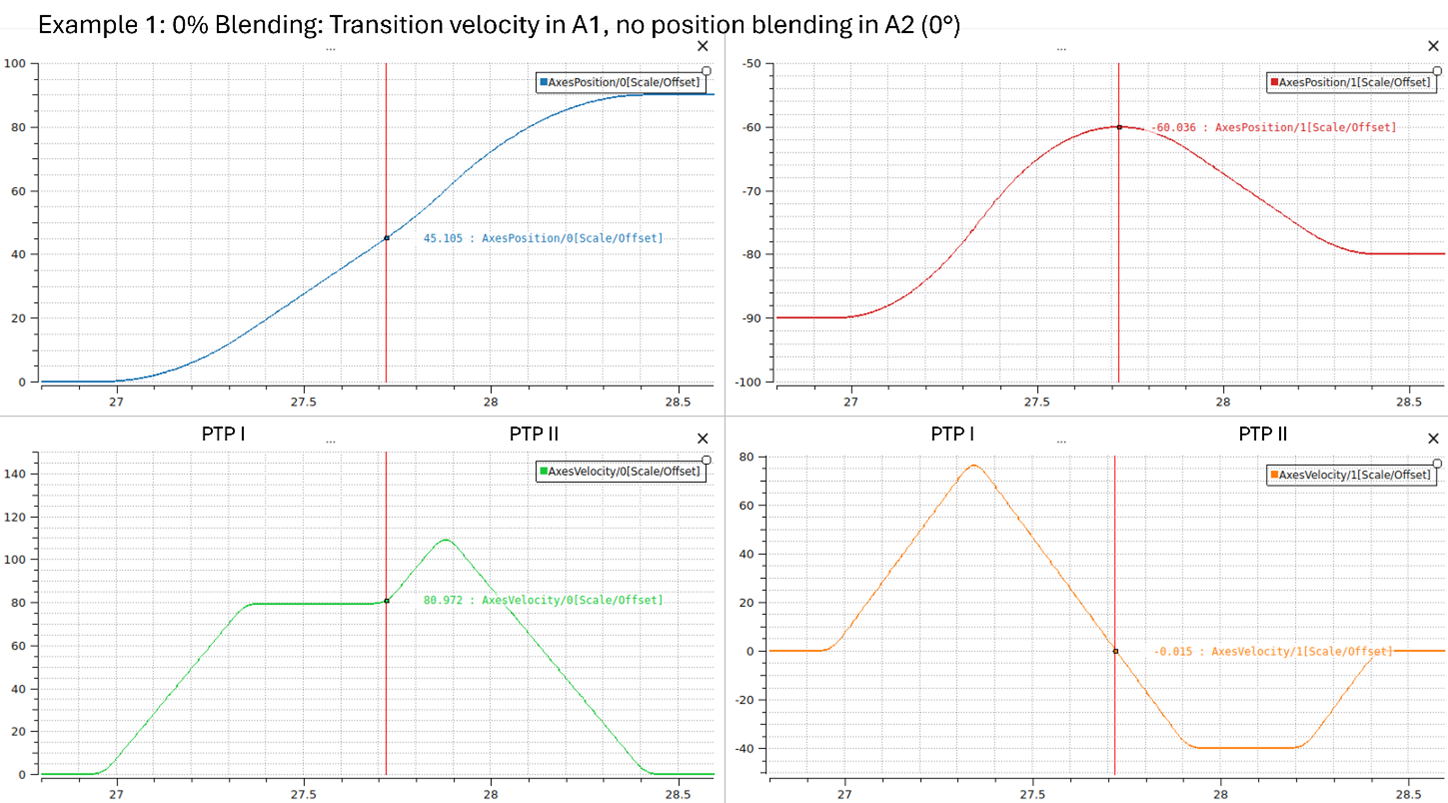
Fig. 20 0% PTP blending, with a transition velocity applied in Axis 1 and no position blending in Axis 2 (0°)
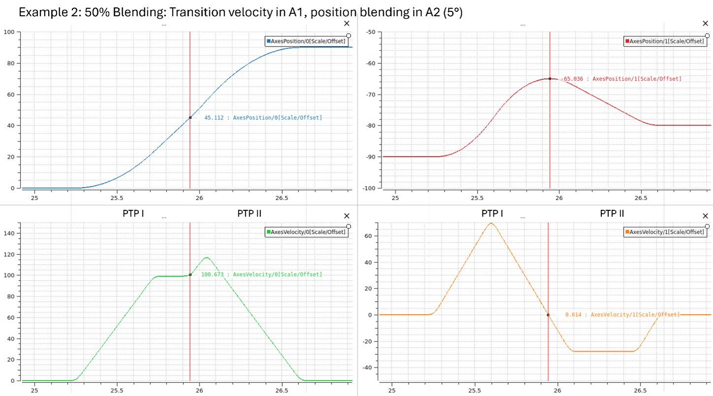
Fig. 21 50% PTP blending, with a transition velocity in Axis 1 and a 5° position blending in Axis 2
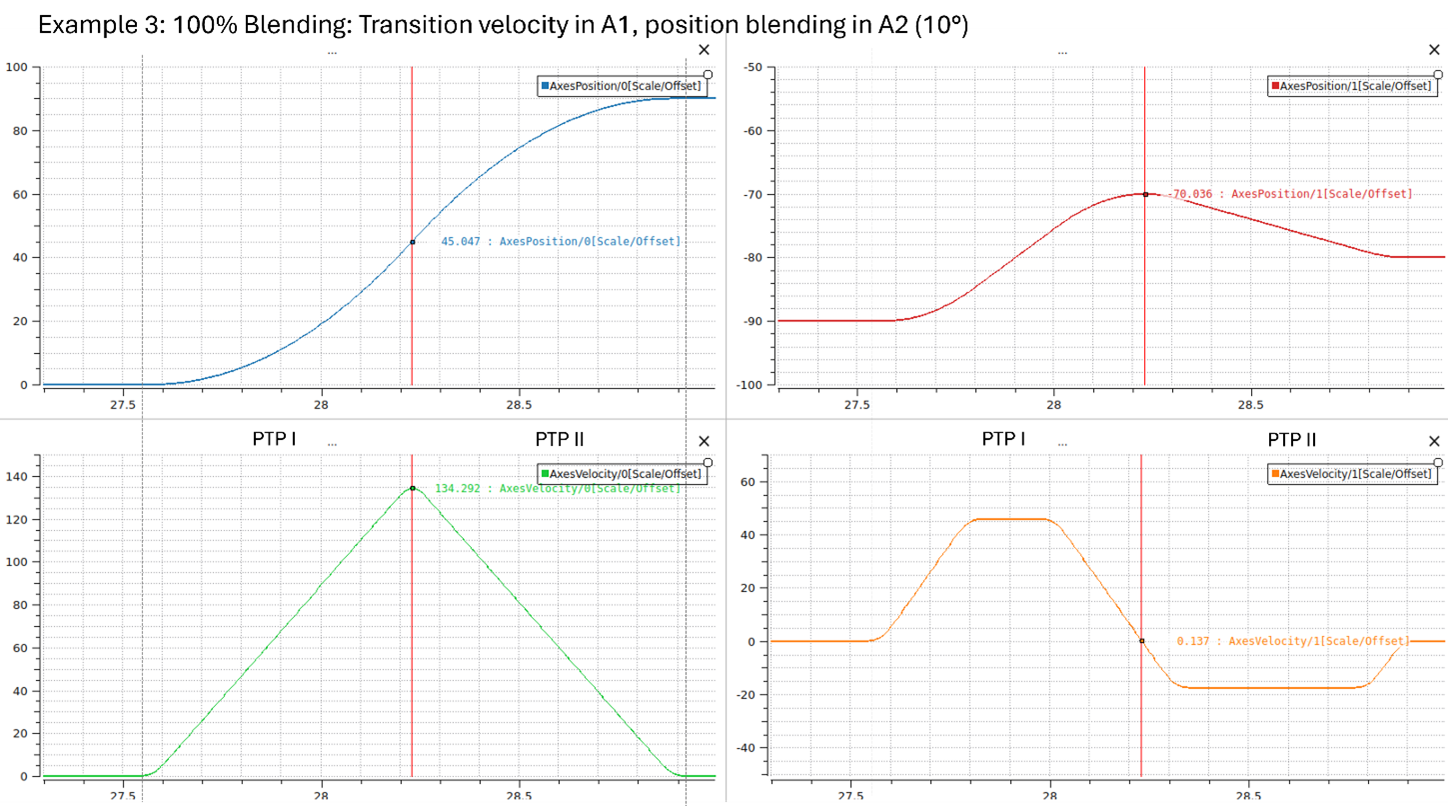
Fig. 22 100% PTP blending, with a transition velocity in Axis 1 and a 10° position blending in Axis 2
4.1.4. PTP-LIN Blending
Note
This feature is currently in a testing stage and therefore disabled by default. It can be activated with the
environment variable VRC_FEAT_CART_PTP_BLENDING: True.
PTP-LIN blending enables smooth transitions between point-to-point (PTP) and linear Cartesian (LIN) motion commands. Unlike pure PTP or Cartesian blending, which operate within a single motion space, PTP-LIN blending bridges joint space and Cartesian space by inserting a combined segment that interpolates between both representations, as seen in Fig. 23.
The blending is bidirectional: it supports transitions from a LIN segment to a subsequent PTP segment as well as from
a PTP segment to a subsequent LIN segment. In both cases, a combined segment
(COMBINED_JOINT_CARTESIAN) is created at the transition point, which internally contains a Cartesian component
and a joint space component.
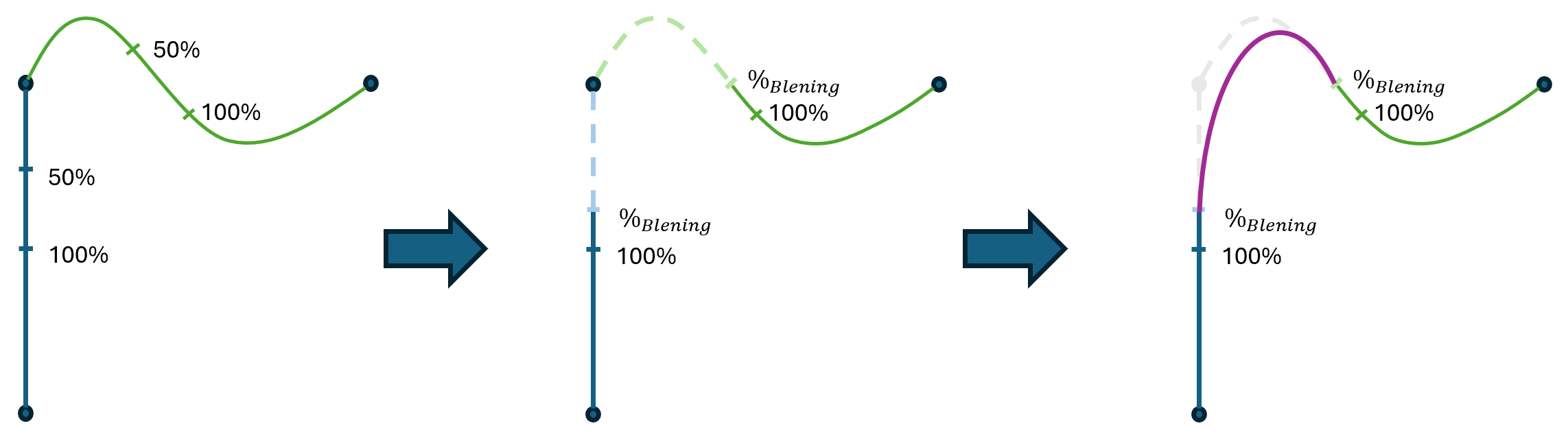
Fig. 23 Schematic of PTP-LIN blending with a combined segment at the transition point
PTP-LIN Blending Parameters
The blending parameter for PTP-LIN blending is specified in the subsequent (requesting) motion command and defines the degree of blending between the two segments. As with Cartesian blending (see Cartesian Blending Parameters), the parameter can be provided either as a percentage or as an absolute value:
Percentage \([\mathrm{\%}]\): The blending radius is calculated as a fraction of half the segment’s path length, analogous to the definitions for Cartesian and PTP blending (see Cartesian Blending Parameters).
Absolute \([\mathrm{m}]\): In absolute blending, the blending distance in the Cartesian segment is converted into a percentage value, which is then also applied in the PTP blending.
Note
PTP-LIN blending is not symmetric: the blending parameter is applied independently to the previous and next segment. This means the blending distance from the transition point may differ on each side.
A key difference to pure Cartesian or PTP blending is that the segments are cut at the blending point independently for the previous and next segment. The cut motion profiles are then transferred as subsegments to the combined motion object: the first subsegment follows the previous command and decelerates to standstill, while the second subsegment starts from standstill and accelerates into the next segment. Both subsegments are interpolated simultaneously within the combined segment (see superposition described above).
Blending Path Geometry
The exact geometry of the blending path is not precisely defined. The blending points indicate where the robot enters and exits the blending zone. It is to be expected that the robot will not leave the original path immediately after the first blending point and may return to the original path before the second blending point.
The actual trajectory depends on several constraints. These include the path length, velocity and acceleration of the adjacent segments, as well as general settings such as the length of the interpolation filters (see System Parameter).
Note
Currently, the time override also affects the path geometry.
In general, slower movements and shorter segments produce a narrower blending segment.
Furthermore, the blending path may differ depending on whether the transition is from LIN to PTP or from PTP to LIN.
Edge Cases for PTP-LIN Blending
This section describes specific situations that require special consideration when using PTP-LIN blending.
Very Short Segments
Currently, problems may arise when very short segments (below \([\mathrm{1°}]\) or \([\mathrm{1cm}]\)) are blended.
Influence of TimeOverride
For PTP/Lin Blending, we have observed that the TimeOverride has little influence on the geometry of the
blending segment.
4.1.5. Blending with Interpolating Segments
In principle, blending can also be used if the previous segment is already interpolating.
However, there is no guarantee that the blending calculation will be successful or that the specified blending parameters can be applied.
Blending attempts to be performed using the remaining segment length (minus a tolerance that is expected to be traveled during path planning).
The success of the blending therefore depends largely on the interpolation progress of the previous segment.
It may also happen that there is no longer enough time left to calculate the blending. This can be the case, particularly with short segments.
Note
Blending performance can depend heavily on whether voraus Robot Control is running on a real-time capable system or not.